and the
FAST OSCILLOSCOPE
Many experiments in physics deal with voltage or charge pulses from radiation detectors or other signal sources. These pulses are often very small and must be amplified without distortion before examination with a Cathode Ray Oscilloscope (CRO) or further processing. Properly connecting a pulse source (the detector) to an amplifier or CRO is not a trivial task, and cannot usually be accomplished by using simple wire clip leads. One usually needs to shield against noise pickup, or maintain the proper impedance (or both simultaneously), while preserving the maximum bandwidth of the signal. This requires the use of compensated attenuator probes or a terminated shielded coaxial cable (transmission line). A pulse must be thought of as a superposition of many high-frequency AC components with the transmission of these components being governed by Maxwell's equations. The salient property of a transmission line is best described by a characteristic impedance. The boundary conditions, imposed by Maxwell's equations, must be respected at each interface (where the transmission line is connected to a source or load), i.e., a transmission line must be correctly terminated at those interfaces to avoid reflections that will distort the signal.
THEORY OF THE TRANSMISSION LINE/COAXIAL CABLE:
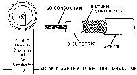
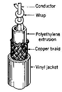
A coaxial cable consists of a central wire that carries the signal (the pulse) and an outer coaxial cylindrical shield that is at ground potential. This shield not only minimizes electromagnetic noise picked up by the central wire, but it constitutes, together with the central wire, a "system" with a unique capacitance and inductance per unit length and a unique velocity of signal propagation. It also exhibits resistance and dispersion. It is the purpose of this experiment to familiarize you with the basic characteristics of coaxial cables and their proper use.
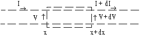
Consider initially a long parallel-wire line of negligible resistance with inductance L per unit length, and capacitance C per unit length.
>
Apply Kirchhoff's laws to the closed path shown :
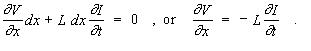 (1)
(1)
The charge per unit length is:
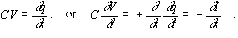 (2)
(2)
Further differentiation leads to the wave equation:
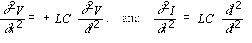 (3)
(3)
It is readily verified that a complete solution for V is given by:
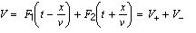 (4)
(4)
representing waves traveling in both positive and negative x-directions, with a velocity of  .
F1 and F2 are arbitrary functions of the arguments t ± x/v. To find the solution for I, we write:
.
F1 and F2 are arbitrary functions of the arguments t ± x/v. To find the solution for I, we write:
 (5)
(5)
Integrating this with respect to t gives:
 (6)
(6)
or
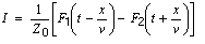 (7)
(7)
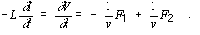
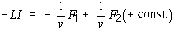
With lines of finite length or with discontinuities, boundary conditions must be fully satisfied, i.e.,
Kirchhoff's laws must apply. Imagine that the impedance changes suddenly from Z0 to Z1 (for example,
a finite line that is terminated with a resistance, or joined to another line of different characteristic
impedance). Then, if we regard the total voltage and current to be made up from forward and reverse
traveling waves, we have at the junction, for Z1 resistive:
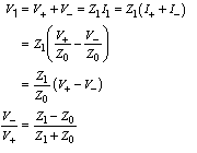
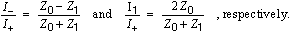
Thus a wave incident on a discontinuity will result in a new wave moving in the reverse direction, the
voltage reflection coefficient being:
(Z1 - Z0) / (Z1 + Z0) (9)
The voltage transmission coefficient will be:
V1 / V+ = (V+ + V_) / V+ = 2Z1 / (Z1 + Z0). (10)
Similarly, the reflected and transmitted currents are given by
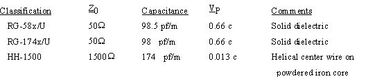
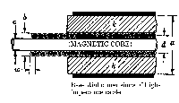
Figure 2. Internal Structure of Selected Coaxial Transmission Lines.
All lines listed have polyethylene insulation with a dielectric constant of 2.3 and a coaxial copper wire sheath (braided for all but HH-1500) with a shielding efficiency of ~ 88-95%. Check the variant letter RG-nn(x), which specifies center conductor material and the jacket and shield properties; differences may be substantial. Parameter values shown are nominal (~ +/- l0%.).
HH-1500 (RG-266) cable achieves a very wide bandwidth, high characteristic impedance, and very low attenuation with a large diameter center conductor (low R) tightly wound on a powdered iron core (mu ~ 100) to obtain a high inductance/unit length and a Velocity of Propagation (VP) of 3.81 m/microsec (c = 300 m/microsec). The outer sheath is a helical wrap of tightly packed parallel insulated copper wires to reduce eddy current losses.
Attenuation is due principally to the resistance of the conductors and is essentially frequency independent, for frequency < 1 MHz. Dielectric and copper (skin effect) losses become significant as frequency increases ( > 10 MHz), with a degradation of fast transitions as higher Fourier components of a pulse are preferentially attenuated. The powdered iron core of the HH-1500 cable shows similar frequency characteristics. Manufacturers supply loss data in db/unit length.
THE CATHODE RAY OSCILLOSCOPE (CRO) AND SIGNAL SOURCES:
In this (or any) laboratory it is necessary that you use the Cathode Ray Oscilloscopes (CRO) competently. (Understanding and skill in using any CRO is undoubtedly the single most valuable laboratory asset you can acquire.) A combination of a wide-band oscilloscope, with either terminated signal cables or compensated attenuator probes, is a powerful and accurate "eye" to you as an experimenter, but only if you understand the ways by which signals may be modified or degraded. Understanding the relationships between the Fourier components of the signal and the rise-time/frequency characteristics of the CRO is essential. The CRO will frequently require the services of signal sources, whose characteristics also must be understood.
Use the "First-Time Operation" sequence found on pages 1-3 to 1-12 of the OPERATORS MANUAL for the Tektronix Model 7603 CRO to familiarize yourself with both the CRO and the signal generators. (This MANUAL is intended for someone unpacking a NEW instrument. Ignore all references to Calibration adjustments.) Concentrate on the fundamentals of the Vertical and Horizontal systems. Study the Specifications and Operating Instructions for the Model 7A15A/AN Amplifier and 7B50 Time Base. Use the Tektronix Model 114 Pulse Generator (PG) connected to the CRO vertical input with RG-58/U cable and a 50 Ohm feedthrough terminator to verify the operation of both units. What changes when the terminator is removed? Investigate the PG Trigger Output/CRO EXTERNAL TRIGGER Input, as well as the behavior of the vertical display. Note well the behavior of the display when you change from AC to DC Input coupling when viewing a low-duty-cycle pulse train. Use the Fairchild Time-Mark Generator to verify that the CRO Time Base meets the manufacturer's sweep-time/linearity accuracy specifications.
Use the Tektronix Model 106 Square-Wave Generator to test the relationship of Rise Time to Band Width for the CRO. Test the rise time (Tr) of the CRO, for both positive- and negative-going transitions, by connecting the Model 106 to the 7A15A input with an RG-58/U cable and a feedthrough 50 Ohm terminator. The Model 106 produces three outputs; two simultaneously at a level of +/- 0.05 to 0.5V with Tr ~ 800 ps, or a third high-level output of ~7 V to > 120 V into 1 MegOhm with Tr < 120 ns, or 0.5 to > 12 V into 50 Ohm with a Tr of < 12 ns. Rise time specifications are valid with the Transition Amplitude controls set near maximum ( > 3 o'clock) Use a repetition rate of 10 to 100kHz, and the CRO 10x sweep MAGNIFIER for easier measurements.
*** CAUTION *** *** IMPORTANT ***
The Tektronix Model 106 is a CALIBRATION instrument, that will be damaged by connecting the Low-Level FAST-RISE outputs to a short-circuit or a reactive load. Connect these outputs only to the input of a CRO, directly or through a 50 Ohm terminator. The HI AMPLITUDE output supplies hazardous voltages (120V) unless it is terminated!
Repeat the risetime measurements using the lx and l0x probes. To do this, remove the RG-58/U cable and attach the 50 Ohm feedthrough terminator directly at the Model 106 output connector. Connect the probe to that terminator using a BNC-to-Probe adapter fitted to the 10x probe's tip. Repeat with a lx probe. Repeat the measurement once more with an unterminated 1 m RG-58/U cable between the generator and CRO. Have you accurately measured the CRO risetime, or should a correction be made for the finite pulse risetime of the Model 106? Check APPENDIX A.
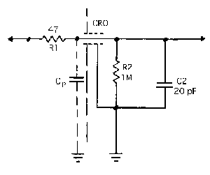
Figure 3. Connection Panel for Coaxial Cable Measurements.
1. Connect a 50 Ohm (RG-58/U) cable from the Model 114 Pulse Generator (PG) to Pl (Fig. 3), with HH-1500 cable between connectors P2a and P3a. Set up the 114 Pulse Generator for positive SQUARE WAVES, maximum output, and connect a l0x probe (pincher tip) to P2a. Initially, use a pulse period of roughly 100 microsec. Set the CRO sweep speed to 5 microsec/cm so as to display only the positive transition of the signal. Use an EXTernal Trigger, i.e., set the CRO for EXTernal Triggering, with the PG TRIG OUT signal set for Leading Edge.
Determine the value of Z0 in two ways, (a) and (b), as follows:
[This arrangement, delay line "clipping", is used to obtain a pulse of short duration while accurately preserving its peak amplitude.] Because the cable is not lossless, the negative traveling wave arriving at P2a, due to reflection at P3a, cannot completely cancel the input positive wave. Measure delay time (50% amplitude) as well as the attenuation coefficient (MKS units). Assume that the required modification to Equation 4 is:
What is the rise time (10% to 90% points) of the 114 Pulse Generator POSITIVE output at Pl? What is the rise time of this transition at P2a? Why are they not the same? What is the fall time of the negative going transition of the square wave at Pl? At P2a? (Try utilizing the PG Leading/Trailing Edge switch.) Are they the same as the corresponding positive transition times? Be certain that you understand what is happening and why.
3. With Rla set to its maximum value (~20,000 Ohm) and the cable disconnected from P3, observe the stepwise rise in voltage at P2a. Use a 1 msec square wave, at least to start. Explain the relative heights of ALL of the FIRST FIVE steps. Determine the time required for the waveform envelope to rise to within l/e of its ultimate value and compare with the rise time [(Rla)(C total)] that would be expected from this simple "integration network". The value of (C total) can be found from the propagation velocity V and your measurement of Z0. You will find it instructive to calculate the number n of transits necessary for:
for the ideal line. Assume that 2nT = (Rla)(C total) since Rla >> Z0. T is the one-way transit time.
** 4. Connect a length of HH-1500 cable between the 114 PG with a right-angle adapter (0.1 ms square wave) and the vertical input of the CRO with another right-angle adapter. What is happening? Next install a 1500 Ohm series resistor at the PG end. What happens? (These resistors are mounted in hexagonal tubes with BNC connectors. The resistor is connected from center pin to center pin, with the outer shell providing only shielding and mechanical support.) What happens if the resistor is at the CRO end? Remove the series R at the PG, and connect a 1500 Ohm resistor from the CRO input to ground, i.e., terminate the cable. (Use a tee and shorting cap.) Describe the effect. Replace the series R at the PG. What is the effect of having both ends of the cable terminated? In every case here, examine the trace at both fast and slow sweep speeds.
** 5. Connect both ends of an HH-1500 cable to P2a with a "T" connector, then adjust Rla for minimal reflections. Explain the pattern seen at P2a and the value of Rla you decide is correct.
** 6. Place a copper cylinder around a length of HH-1500 cable connected from P2a to P3a (Set Rla = Z0, and R2a = 0 ). Explain the pattern at P2a as the cylinder is moved along the cable. (Hint: look for small movable artifacts on both the top and trailing baseline of the pulse.)
** OPTIONAL.
* Primary reference, available as copies in the reference binder at the experiment.
Copies of the reference binder are available for OVERNIGHT signout. Additional material will be found at the experiment setups.
Three parameters are used to describe the capabilities of any oscilloscope: sensitivity, risetime (Tr), and bandwidth (3 db BW). The last two, and their relationship, will be discussed here. Bandwidth is the frequency span between points where the response is reduced to 70.7% (- 3db) of the level at mid frequencies.
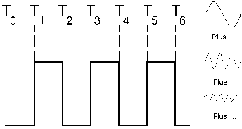
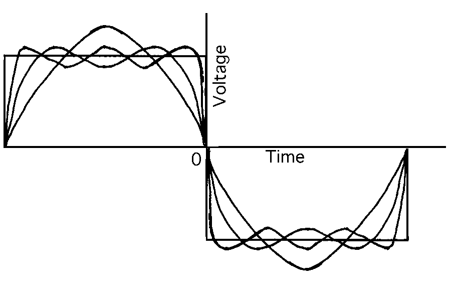
Consider the ideal periodic wave train (Fig. A-l) with instantaneous transitions from low/high, or high/low. It can be resolved into its Fourier components, a set of sine waves of the correct frequency, amplitude, and phase. The lowest frequency equals the repetition rate, while the higher harmonics, when added with correct amplitude and
Figure A-1. Ideal pulse train and lower order Fourier components.
phase, sharpen up the transitions and flatten the horizontal sections. A "perfect" square wave contains harmonics to infinity.
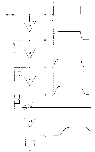
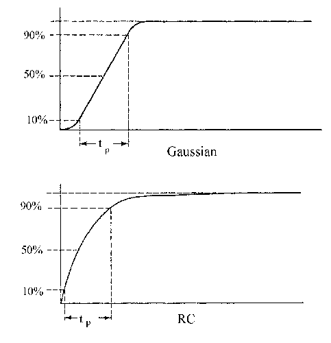
Any network, passive or active, will modify this ideal pulse. When square waves are applied to a simple RC integrator, the output transitions have the shape shown in Fig. A-2: the common exponential curve, most easily characterized by its "risetime", the time required to go from 10% to 90% of maximum amplitude. It requires 0.1 RC to move from 0 to 10%, and 2.3 RC to reach 90%, hence the 10% to 90% time is 2.2 RC. It is more common to have networks of many stages, such as the multi-stage amplifier chain in a CRO. When an ideal square wave passes through n identical stages similar to Al (Figure A-2), the leading edge is delayed, slowed down, and changed in shape by each stage. If n is large (3-5 for practical purposes), the leading edge approaches a Gaussian shape. See Figure A-3 for a comparison of the simple RC and Gaussian shaped pulses. The RC pulse rises abruptly, almost linearly, from 0 to 10%, then requires as much time to go from 90% to 99% as from 0 to 90%. The Gaussian response rises from 0 to 10% more slowly, then becomes almost linear up to 90% and the takes as much time to go the last 10% as for the first 10%. The top corner is the mirror image of the bottom corner.
Figure A-2. Effect of n networks.
Figure A-3. RC and Gaussian pulses.
The relationship between a Gaussian shaped pulse and bandwidth is more complicated than for the RC case, since the network bandwidth of the network(s) must be folded in.
This relationship is completely valid only for networks with a bandwidth that is RC limited, a reasonable assumption for most modern CRO's. When an ideal pulse passes through n devices in cascade, each will contribute to the increase in risetime a predictable manner. The displayed rise time (Tr) , where Trpg is the risetime of the pulse generator, will be:
It is customary to adjust CRO vertical amplifiers for best pulse response, i.e., for fastest risetime with the minimum of top corner overshoot. The risetime/bandwidth product typically varies from 0.32 (about 5% overshoot), to 0.37 ( < l% overshoot). From the practical standpoint, the CRO must have a risetime about 5 times faster than the pulse being examined to insure measurement errors of less than 2%.
Signals may be connected to the input of a CRO in a variety of ways. Care must be exercised if serious distortion of the signal is to be avoided. Because it is not always possible to use a terminated cable, several types of voltage probes have been developed. The most common are the lx straight through, and l0x attenuating probes.
This is NOT a length of coaxial cable with convenient connectors at each end! It has a special low capacity cable (6.5 pf/ft, Z0 = 265Ohm) with a resistive center wire (R = 265Ohm) providing the correct termination to the system for the duration of reflections of the leading edge of fast rise signals.
Figure B-1 Typical 1x Straight through Voltage Probe.
Circuit loading is 1 Megohm resistive (CRO input R) in parallel with the CRO input capacitance (20 pf) + the 6.5 pf/ft of the probe cable (70 pf total). The "center wire termination" limits useful bandwidth to < 30 MHz. An ordinary coaxial cable has a higher capacitance of 13 to 29 pf/ft, and shows heavy ringing or standing waves (low center wire R) when used with fast or high frequency signals. Test this.
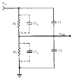
This device provides lowered circuit loading at the cost of reduced sensitivity. It is a frequency compensated 10:1 voltage divider. See Figure B-2. Rl is a 9 MegOhm miniature resistor located at the probe tip, while R2 is the 1 MegOhm input resistor of the CRO vertical input. The resistors are a precise (1%) 10:1 voltage divider at DC, with the capacitor C1s being the stray capacitance at Rl, while C2s consists of the probe cable capacitance + strays. (The cable used is the same as described for the lx probe.) The unavoidable stray and cable capacitance produces increasing loading (errors) with increasing frequency. To hold the attenuation ratio constant with increasing frequency, Cl is added to shunt Rl to the same extent that C2 (CRO input C + cable capacitance + a small variable capacitor) shunts R2. If the ratio of the reactances of Cl:C2 is exactly 9:1 the response of the probe will be flat to the upper BW limit, preserving the shape of fast pulses with minimal aberrations. "Compensating" a probe is simply adjusting this ratio.
Figure B-2 10x Attenuating Probe circuit.
The Lab's l0x probes load the circuit under test with 10 MegOhm in parallel with 13 pf. The bandwidth is > > l00Mhz with a risetime short enough so as to not degrade the performance of a CRO rated at Tr < 3.5 ns.
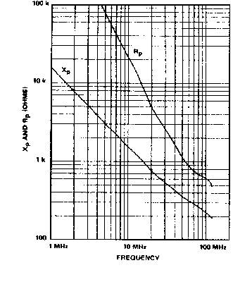
Since this is a compensated RC attenuator, the attenuation ratio remains constant while the impedance presented to the circuit under examination drops with increasing frequency. See Figure B-3. Voltage derating is required as frequency increases because of the lowered reactance of the capacitive components, heating, and voltage breakdown.
Figure B-3 Frequency-Impedance Characteristics of a 10x Probe.
 is called the characteristic impedance of the line, and is a pure resistance for an ideal
(lossless) line. (Note that the relationship between voltage and current for a forward traveling wave is
V+ /I+ = Z0 and for the reverse wave V_ /I_ =-Z0. Take care not to confuse the propagation direction
with the direction of the current; positive current is to the right.) Thus the terminals of an infinitely
long parallel-wire transmission line behave in a circuit as a pure resistance Z0.
is called the characteristic impedance of the line, and is a pure resistance for an ideal
(lossless) line. (Note that the relationship between voltage and current for a forward traveling wave is
V+ /I+ = Z0 and for the reverse wave V_ /I_ =-Z0. Take care not to confuse the propagation direction
with the direction of the current; positive current is to the right.) Thus the terminals of an infinitely
long parallel-wire transmission line behave in a circuit as a pure resistance Z0.
 (8)
(8)
 (11)
(11)
EXPERIMENTAL TASKS
Similar precautions ARE NOT required when using the Tektronix Model 114 Pulse Generator. It has circuitry installed to protect the output devices at the cost of a longer transition time of 10 ns. TRANSMISSION LINE MEASUREMENTS:
2. Measure the characteristic impedance, velocity of propagation, and attenuation coefficient for the other samples of coaxial cable available (either RG-58/U or RG-174/U). (Use Rlb only, with a shorting cap at far end.) Consult manufacturer's data regarding Z0, VP, and attenuation for the HH-1500, RG-58/U or RG-174U. Tabulate both "book values" and your measured values. 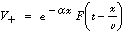

QUESTIONS
REFERENCES
APPENDIX A
BANDWIDTH - RISETIME RELATIONSHIPS:


APPENDIX B
1x PROBE:
10x ATTENUATING PROBE: